A Guide to Auto ABS Loss Curve Modeling

Forecasting credit losses in auto loan portfolios is a core discipline in structured finance. For analysts, auto ABS loss curve modeling is the primary tool for predicting the timing and severity of defaults, which directly informs security pricing, risk management, and credit ratings. This isn't just an academic exercise; it's a critical workflow for anyone pricing or monitoring asset-backed securities. This guide explains the data lineage behind building these models—from sourcing raw remittance data in public filings to applying robust modeling techniques. The goal is a transparent, defensible, and reproducible analytical process. With platforms like Dealcharts, analysts can visualize and cite the underlying performance data, connecting model assumptions directly back to their source.

Market Context: Why Loss Curves are a Moving Target

The auto ABS market is a dynamic ecosystem, heavily influenced by economic cycles, consumer behavior, and underwriting standards. A loss curve model built on data from a stable economic period will fail catastrophically during a downturn if it isn't calibrated to reflect changing market conditions. This is why a "set it and forget it" approach is inadequate; models must be continuously monitored and adjusted.

A key challenge is the variability in loan performance across different originators and economic environments. For example, market-shaping trends in subprime auto ABS show how underwriting standards can loosen during competitive periods, leading to higher-than-expected defaults. The model must account for the specific underwriting environment of the loan vintage it analyzes. Macroeconomic factors like unemployment rates, GDP growth, and used vehicle values—tracked by indices like the Manheim Used Vehicle Value Index—are also critical inputs. A verifiable model must link these external factors to observable performance data from filings.

Data Foundation: Sourcing and Structuring Remittance Data

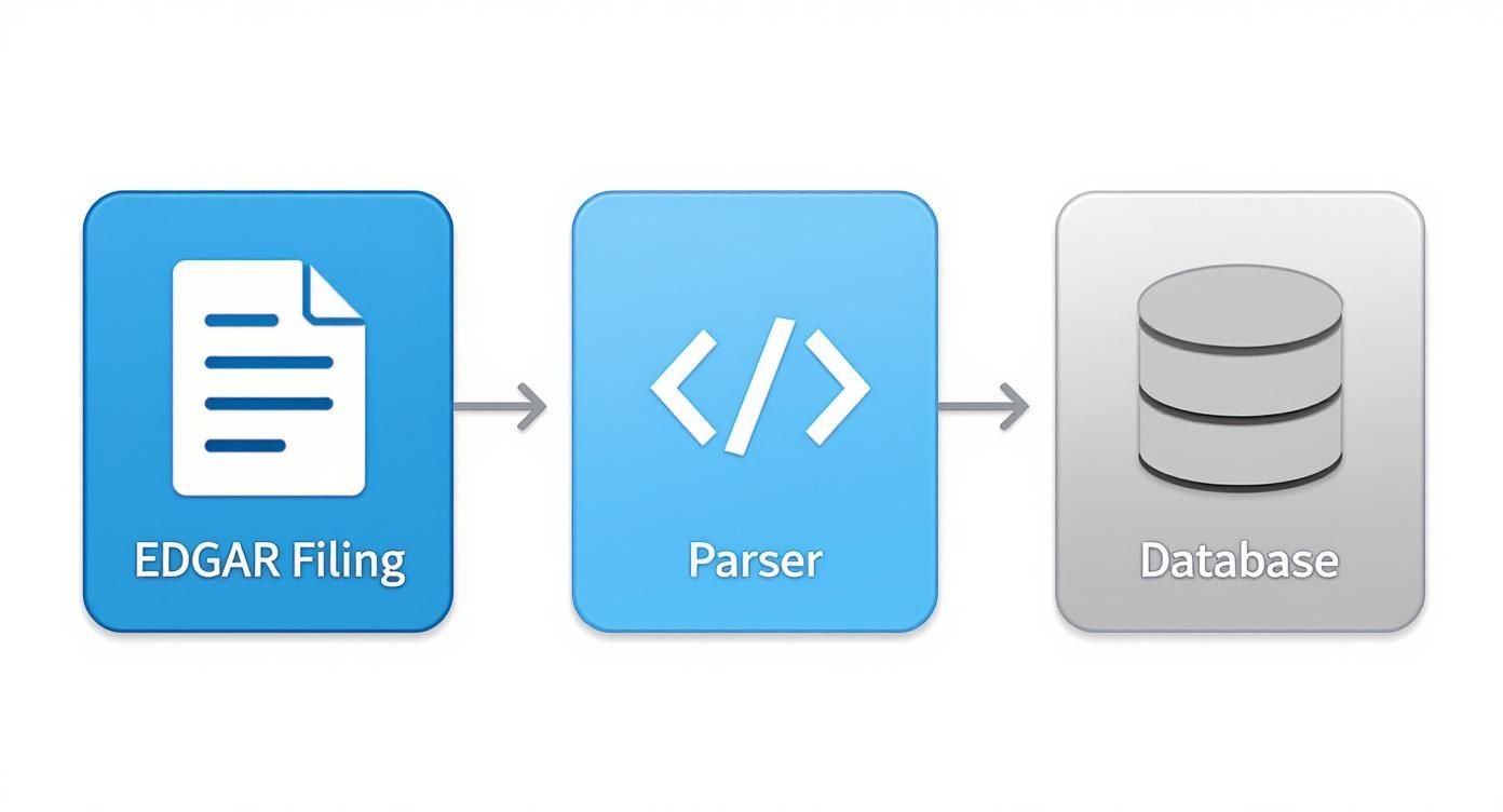
A robust auto ABS loss curve model is built on a foundation of verifiable, high-quality data. The primary sources are public regulatory filings submitted to the SEC's EDGAR database. The two most critical documents are the 424B5 prospectus, which details the initial collateral pool statistics, and the monthly 10-D remittance reports, which provide ongoing performance data like delinquencies, defaults, and recoveries.

For data engineers and analysts, the main technical challenge is programmatically accessing, parsing, and structuring the data from these filings. The information is often embedded in unstructured text or non-standardized HTML tables, with formatting that can vary even for the same issuer across different deals. The workflow involves:

1. Fetching Filings: Using the EDGAR API to systematically download 10-D and 424B5 filings for a target universe of auto ABS deals.
2. Parsing Tables: Writing scripts (e.g., in Python with libraries like BeautifulSoup or lxml) to extract key performance tables containing static pool data, delinquency roll rates, and cumulative net loss (CNL) figures.
3. Structuring and Linking: Normalizing the extracted data and storing it in a structured database, ensuring each data point is linked to its deal (via CUSIP or CIK), vintage, and reporting period.

This data plumbing is a significant undertaking. This is precisely why platforms like Dealcharts, which provide pre-parsed and linkable datasets, are so valuable. They handle the extraction and structuring, allowing analysts to focus on modeling rather than data wrangling.

Example Workflow: From Raw Data to a Loss Projection

Let's walk through a simplified, programmatic workflow for building a loss curve using Python. This example highlights the data lineage from source to insight. The core idea is to use historical performance from seasoned deals to project the future performance of a newer, unseasoned deal.

First, we wrangle historical cumulative net loss (CNL) data for multiple vintages from a specific issuer, which we've parsed from 10-D filings. The goal is to create a clean, normalized dataset where losses are tracked by the age of the loan pool (months on book).

# --- Python Snippet: Calibrating a Loss Curve ---
# Assume 'df_historical_cnl' is a pandas DataFrame with CNL data
# sourced from parsed 10-D filings.
# Columns: ['vintage', 'months_on_book', 'cnl']

import pandas as pd
from scipy.optimize import curve_fit
import numpy as np

# 1. Define a functional form for the loss curve (e.g., Weibull CDF)
# This mathematical function will model the S-shaped loss curve.
def weibull_cdf(x, k, lmbda):
    """Weibull cumulative distribution function."""
    return 1 - np.exp(-(x / lmbda)**k)

# 2. Select a representative historical vintage to create a base curve
# Data lineage: This vintage is chosen based on similar collateral characteristics
# found in the 424B5 prospectus of our target deal.
base_vintage_data = df_historical_cnl[df_historical_cnl['vintage'] == 'DRIVE 2022-1']
x_data = base_vintage_data['months_on_book']
y_data = base_vintage_data['cnl'] / base_vintage_data['cnl'].max() # Normalize to 1

# 3. Calibrate the model by fitting the Weibull function to historical data
# The optimization finds the parameters that best describe the historical loss timing.
params, _ = curve_fit(weibull_cdf, x_data, y_data, p0=[2, 30])
k_fit, lmbda_fit = params
print(f"Fitted Weibull Parameters: k={k_fit:.2f}, lambda={lmbda_fit:.2f}")

# 4. Project the full curve for a new deal using the fitted shape
# Data lineage: The 'lifetime_loss_assumption' is an analyst's projection
# informed by early performance of the new deal and macro forecasts.
lifetime_loss_assumption = 0.05 # 5% Cumulative Net Loss
months_to_project = np.arange(1, 73) # Project for 6 years
projected_cnl = lifetime_loss_assumption * weibull_cdf(months_to_project, k_fit, lmbda_fit)

print("\nProjected CNL for new deal:")
print(pd.Series(projected_cnl, index=months_to_project).head())

This workflow demonstrates explainability. The final projection for a new deal is directly traceable to:

1. Source: Raw 10-D remittance reports for a specific historical deal (e.g.,

   DRIVE 2022-1

   ).
2. Transform: A mathematical model (Weibull CDF) is calibrated to this historical data.
3. Insight: The calibrated model is applied to a new pool with an explicit lifetime loss assumption, generating a verifiable forecast. You can explore the final remittance data for a deal like the DRIVE 2025-2 trust to see what this structured output looks like.

Insights and Implications for Modern Analytics

Embedding verifiable data lineage into the modeling process transforms a black-box forecast into a transparent analytical tool. This "model-in-context" approach, a core theme of CMD+RVL, provides several advantages for risk monitoring and advanced analytics. When a deal's actual performance deviates from the forecast, an analyst can immediately trace the variance back to its source—was it a flawed assumption about recovery rates, or are delinquency roll-rates from the latest 10-D simply higher than historical precedent? This explainable pipeline makes analysis defensible to risk committees, investors, and regulators.

Furthermore, this structured context is essential for building more advanced systems. For example, a Large Language Model (LLM) connected to a graph of linked data (filings, deals, performance metrics) can reason about model outputs. An analyst could ask, "Why did the projected CNL for VALET 2025-1 increase by 30 basis points this quarter?" An LLM with access to the model's lineage could generate a data-backed explanation, pointing to a spike in 60-day delinquencies reported in the most recent remittance report. This moves beyond simple prediction to auditable, automated insight generation.

How Dealcharts Helps

Dealcharts connects these datasets—filings, deals, shelves, tranches, and counterparties—so analysts can publish and share verified charts without rebuilding data pipelines. By providing structured, linkable data extracted directly from source filings, Dealcharts enables users to build, validate, and share models with complete data lineage. This accelerates the path from raw data to defensible insight, allowing teams to focus on analysis rather than data janitorial work. Explore our datasets and tools at https://dealcharts.org.

Conclusion

Effective auto ABS loss curve modeling is not just about statistical accuracy; it's about building a transparent and explainable analytical process. By grounding models in a clear data lineage that traces every assumption back to its source filing, analysts can create forecasts that are not only predictive but also auditable and defensible. This commitment to data context and reproducibility, a cornerstone of the CMD+RVL framework, is essential for navigating the complexities of modern credit markets and building more intelligent financial systems.

Article created using Outrank