Tracking Auto ABS 30/60/90 Delinquencies from 10-D Filings

For structured-finance analysts, monitoring Auto ABS 30/60/90 delinquencies is fundamental to credit surveillance. These metrics, sourced from monthly servicer reports, represent the percentage of loans that are 30, 60, or 90+ days past due. A sustained increase in these figures is a primary indicator of borrower stress and a leading signal for future credit losses. Programmatic analysis of this data, extracted from remittance reports filed as exhibits to SEC 10-D filings, is essential for building accurate risk models and maintaining real-time market awareness. Visualizing these trends through platforms like Dealcharts provides a verifiable, citation-ready view into a deal's underlying performance, directly linking remittance data to actionable insights.

Market Context: Prime vs. Subprime Performance Divergence

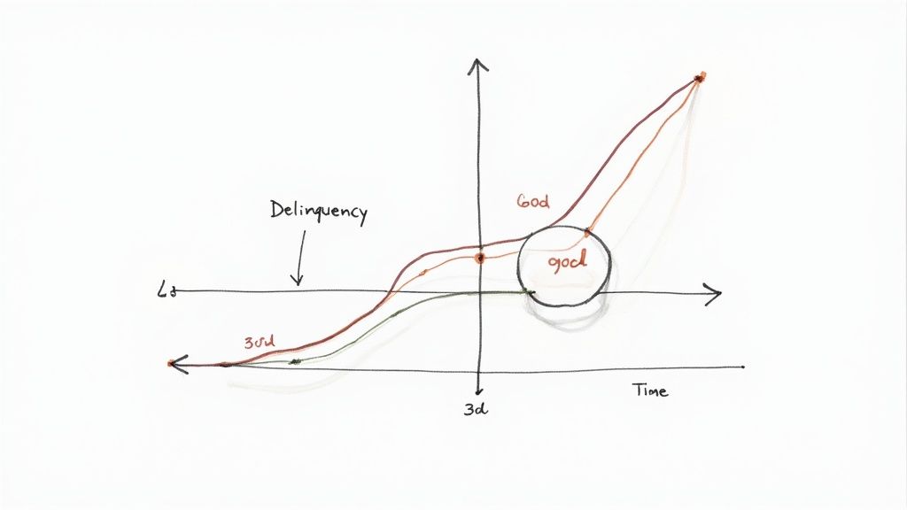
To accurately interpret Auto ABS 30/60/90 delinquencies, one must first understand the current market bifurcation. Economic pressures are not affecting all borrowers uniformly, leading to a significant performance gap between prime and subprime auto loan portfolios.

Recent data shows subprime auto ABS delinquencies have risen to 16%, a level signaling considerable stress among lower-credit-quality borrowers. In contrast, prime delinquencies remain stable at 1.9%. This divergence is a critical source of risk; an analyst examining only blended portfolio metrics could easily overlook the escalating credit deterioration within the subprime cohort. You can read more on these credit market trends for a detailed breakdown. This context is essential for building predictive loss models, particularly when segmenting performance by ABS vintage cohorts.

Data Sourcing: From EDGAR 10-D Filings to Structured Metrics

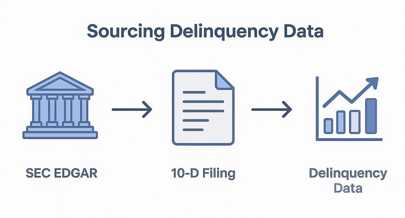
The definitive source for delinquency data is the monthly servicer report, filed as an Exhibit (typically EX-102) to Form 10-D on the SEC's EDGAR system. Programmatic access requires a multi-step process: identifying an issuer's Central Index Key (CIK), querying the EDGAR API for its 10-D filings, and then parsing the attached XML or text-based exhibits.

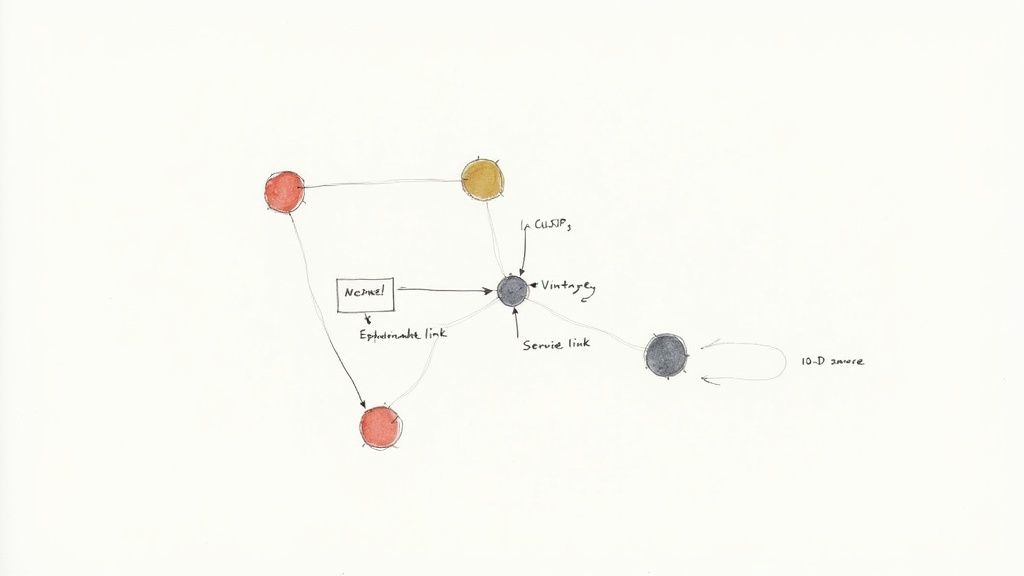
A significant technical challenge is the lack of standardization. Servicers use inconsistent labels for delinquency buckets—for example, "30-59 Days Delinquent" versus "60-89 Days"—requiring robust parsing logic to normalize the data. A reproducible data pipeline follows a clear lineage: CIK → 10-D Filing → Exhibit 102 → Delinquency Table. Once extracted and structured, this data can be linked to other identifiers like bond CUSIPs to create a comprehensive surveillance database. This process has been applied to normalize data for deals like the Element Fleet 2024-1 issuance.

Example: A Programmatic Workflow for Calculating Delinquency Rates

Once raw data is extracted from a 10-D exhibit, the next step is calculating the delinquency rates. The formula is straightforward, but precision is critical. The numerator is the principal balance of loans within a specific delinquency bucket (e.g., 30-59 days past due). The denominator is the current total outstanding principal balance of the collateral pool for that reporting period. A common error is using the original pool balance, which fails to account for amortization and will skew the calculation.

Here is a simplified Python snippet demonstrating the extraction and calculation logic after parsing a remittance file into a dictionary format.

# Assume 'remittance_data' is a parsed dictionary from a 10-D exhibit
def calculate_delinquency_rates(remittance_data: dict) -> dict:
    """
    Calculates 30, 60, and 90+ day delinquency rates from parsed remittance data.
    
    Data lineage:
    Source -> EDGAR 10-D, Exhibit 102
    Transform -> Parsing text/XML to structured dict, calculating rates
    Insight -> Standardized delinquency metrics
    """
    # Denominator: Current outstanding pool balance
    current_pool_balance = remittance_data.get('ending_principal_balance', 0)
    
    if current_pool_balance == 0:
        return {'30_day_dq': 0, '60_day_dq': 0, '90_plus_day_dq': 0}

    # Numerators: Balances for each delinquency bucket
    dq_30_59 = remittance_data.get('principal_balance_30_59_days_delinquent', 0)
    dq_60_89 = remittance_data.get('principal_balance_60_89_days_delinquent', 0)
    dq_90_plus = remittance_data.get('principal_balance_90_plus_days_delinquent', 0)

    # Calculate rates
    rates = {
        '30_day_dq': (dq_30_59 / current_pool_balance) if current_pool_balance else 0,
        '60_day_dq': (dq_60_89 / current_pool_balance) if current_pool_balance else 0,
        '90_plus_day_dq': (dq_90_plus / current_pool_balance) if current_pool_balance else 0,
    }
    
    return rates

# Example usage:
# parsed_data = {'ending_principal_balance': 500_000_000, 
#                'principal_balance_30_59_days_delinquent': 5_000_000}
# delinquency_metrics = calculate_delinquency_rates(parsed_data)
# print(f"30-Day Delinquency Rate: {delinquency_metrics['30_day_dq']:.2%}")
# Expected Output: 30-Day Delinquency Rate: 1.00%

This workflow creates a verifiable data pipeline, ensuring that every metric can be traced back to its source document. Outputs can then be fed into automated reporting tools or used for more advanced modeling.

Implications for Modeling and Explainable AI

Structured, source-linked delinquency data enables sophisticated cohort and vintage analysis. Instead of tracking a single aggregated metric, analysts can compare the performance curves of different loan vintages, linking credit trends directly to the underwriting standards prevalent at the time of origination.

This contextual data is invaluable for machine learning models. Feeding a model not just the delinquency rate, but also the deal CUSIP, vintage, and servicer creates a "model-in-context." The model learns from relationships, not just isolated data points. This approach transforms raw data into an interconnected knowledge graph, making AI-driven insights explainable. When a model flags an anomaly, the analyst can trace its reasoning back to the source 10-D filing, turning a black-box prediction into a verifiable, auditable insight. This is a core theme of CMD+RVL's work on context engines. Properly structuring your analysis presentations is then key to communicating these verifiable findings.

How Dealcharts Accelerates Surveillance

The workflow of sourcing, parsing, and normalizing remittance data is a well-known bottleneck for quantitative analysts. It is time-consuming, repetitive, and prone to error. Dealcharts was built to eliminate this friction. Instead of building and maintaining EDGAR parsers, analysts can access clean, structured time-series data on Auto ABS 30/60/90 delinquencies across thousands of deals. Dealcharts connects these datasets—filings, deals, shelves, tranches, and counterparties—so analysts can publish and share verified charts without rebuilding data pipelines. Every data point is linked to its source filing, as seen in this DRIVE 2025-1 deal example, providing complete data lineage and freeing analysts to focus on generating alpha, not wrangling data.

Conclusion

Mastering the analysis of Auto ABS 30/60/90 delinquencies requires a clear understanding of data lineage—from the raw 10-D filing to the final, calculated metric. A programmatic approach ensures reproducibility and scalability, while context from vintage and issuer data provides the depth needed for robust modeling. This combination of verifiable data and contextual enrichment, a principle central to the CMD+RVL framework, is what enables truly explainable finance analytics and transforms raw numbers into strategic intelligence.

Article created using Outrank