Programmatic Analysis of CMBS Geographic Concentration by State

Analyzing CMBS geographic concentration by state is a critical workflow for structured-finance analysts and data engineers monitoring portfolio risk. While a top-10 state exposure list offers a surface-level view, a programmatic approach is required to quantify idiosyncratic risks tied to local economic shocks, regulatory changes, or regional climate events. This guide demonstrates how to trace loan-level geographic data from its source in SEC filings to a verifiable, model-ready insight. We will cover the data lineage, a practical workflow with code, and the implications for risk modeling. Visualizing this data is straightforward with tools like Dealcharts, which connects raw filing data to deal-specific analytics.

Market Context: Why Geographic Concentration Matters

Geographic concentration in a CMBS deal is a direct byproduct of commercial real estate activity. States with dominant economic hubs and high property values, such as New York and California, consistently anchor CMBS pools. While issuers aim for diversification, the reality is that the most valuable commercial properties are clustered in a few key economic zones, a trend visible across recent CMBS vintages.

This concentration introduces specific, non-diversifiable risks. A deal heavily exposed to Florida is inherently long coastal insurance costs and hurricane risk. A portfolio concentrated in California is exposed to seismic events and the technology sector's cyclicality. As forecasts in the full 2025 CMBS sector outlook call for increased issuance alongside rising delinquencies, quantifying these state-level drivers becomes essential for accurate credit surveillance and stress testing.

Data Lineage: From SEC Filings to State-Level Metrics

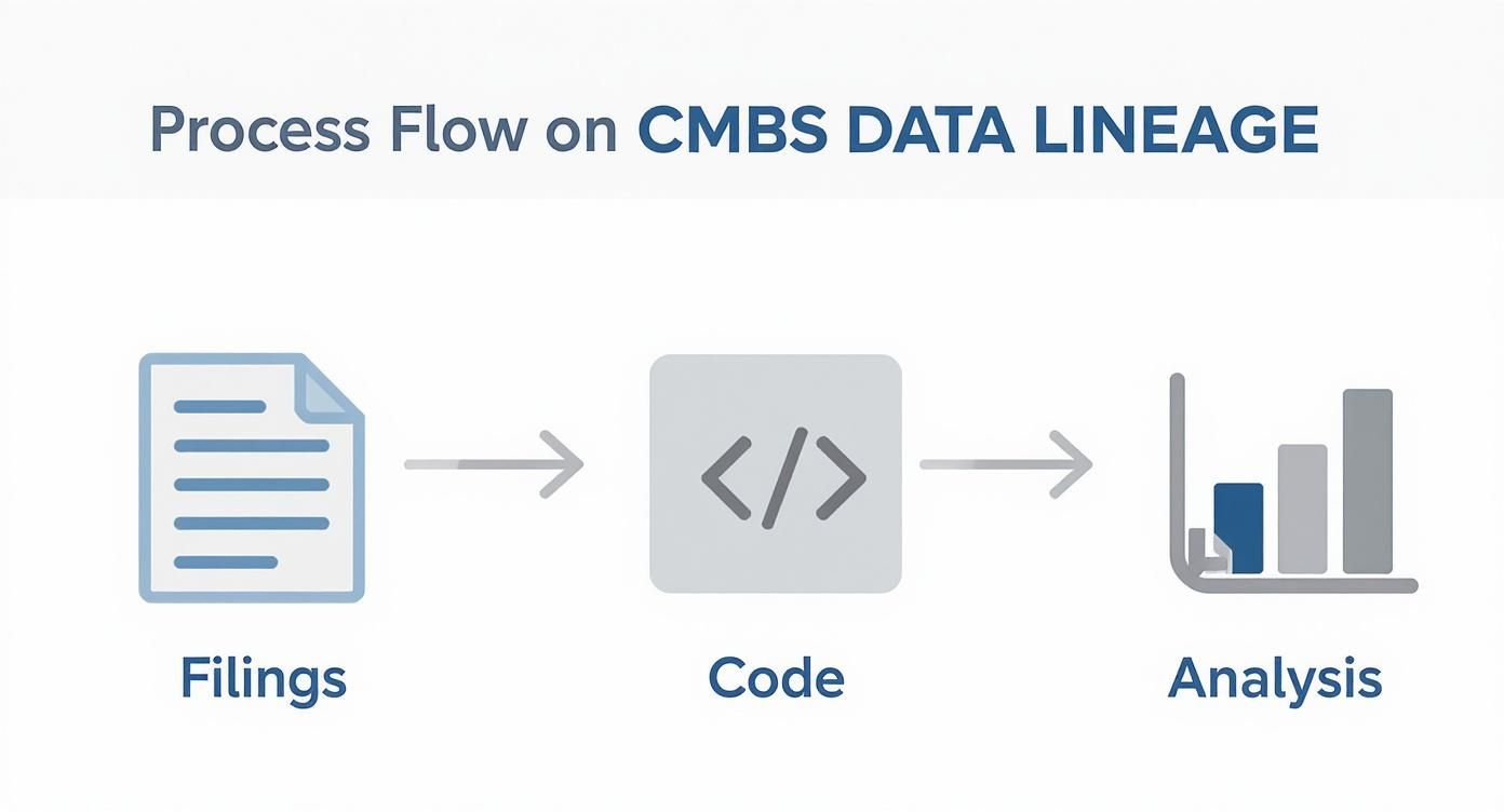
To analyze CMBS geographic concentration by state programmatically, analysts must trace data from source to model. The ground truth resides in loan-level data tapes found within servicer reports (CREFC IRPs) and initial deal prospectuses (424B5 filings). These documents, available via the SEC's EDGAR system, contain the property-level city and state data required for aggregation.

Data engineers can access this information programmatically from EDGAR or commercial data feeds. The core challenge is parsing unstructured or semi-structured formats, standardizing location data (e.g., "NY" vs. "New York"), and linking it to loan balances. Adhering to data integration best practices is critical to ensure a clean, reliable dataset. This pipeline—from raw filing to structured output—is the foundation for any defensible risk analysis, whether for a single deal or an entire vintage like the 2020 CMBS vintage.

Example Workflow: Calculating State Concentration with Python

This section provides a reproducible example of transforming raw loan-level data into concentration metrics. The workflow follows a clear data lineage: source data → programmatic transformation → quantitative insight.

Assume we have a pandas DataFrame

loan_tape

unpaid_principal_balance

property_state

import pandas as pd

# Assume 'loan_tape' is a DataFrame loaded from a parsed servicer report
# loan_tape = pd.read_csv('loan_level_data.csv')

# Step 1: Aggregate Unpaid Principal Balance (UPB) by state
state_concentration = loan_tape.groupby('property_state')['unpaid_principal_balance'].sum().reset_index()
state_concentration.rename(columns={'unpaid_principal_balance': 'total_upb'}, inplace=True)

# Step 2: Calculate total deal balance and each state's percentage share
total_deal_upb = state_concentration['total_upb'].sum()
state_concentration['percentage_share'] = (state_concentration['total_upb'] / total_deal_upb) * 100

# Step 3: Calculate the Herfindahl-Hirschman Index (HHI) for geographic diversification
# HHI is the sum of the squared percentage shares (represented as whole numbers)
state_concentration['hhi_contribution'] = (state_concentration['percentage_share'])**2
hhi_deal = state_concentration['hhi_contribution'].sum()

# Display the results, sorted by concentration
print("Deal Geographic HHI: {:.2f}".format(hhi_deal))
print(state_concentration.sort_values(by='total_upb', ascending=False).head())

This script transforms raw data into a clear, explainable table of state exposures and calculates the HHI, a standard measure of market concentration. This transparent workflow is the bedrock of any trustworthy risk model.

Implications for Risk Modeling and LLMs

Structuring geographic concentration data has significant implications for both traditional credit modeling and emerging AI applications. By connecting a deal's CUSIP to a vector of state-level economic indicators (e.g., unemployment rates, GDP growth, property price indices), analysts can build more dynamic, context-aware risk models. This approach moves beyond static analysis to enable forward-looking stress tests based on regional economic scenarios.

This structured context is also critical for enhancing Large Language Model (LLM) reasoning in finance. An LLM query like, "Summarize the key geographic risks for the MSC 2022-L8 deal," requires a knowledge graph connecting the deal CIK to its underlying properties and their state locations. This is a core principle of CMD+RVL: providing a "model-in-context" where AI can reason over verifiable, interconnected financial data. Without this explainable pipeline from filing to insight, outputs remain unreliable black boxes. The SEC research on CMBS market concentration patterns further validates the importance of this granular data.

How Dealcharts Accelerates This Workflow

Manually building and maintaining the data pipelines required to analyze CMBS geographic concentration by state is resource-intensive. Dealcharts was built to solve this problem by providing a verified, structured environment for CMBS data. Instead of parsing raw servicer reports, analysts can access pre-calculated state exposures for any deal on demand. This allows teams to visualize geographic risk for transactions like MSC 2022-L8 in seconds. Dealcharts connects the critical datasets—filings, deals, shelves, tranches, and counterparties—so analysts can publish and share verified charts without rebuilding data pipelines.

Conclusion

Programmatic analysis of CMBS geographic concentration moves beyond simple reporting to create durable risk intelligence. By establishing a transparent data lineage from source filings to quantitative metrics like HHI, analysts build explainable and reproducible workflows. This approach not only strengthens credit risk models against localized economic shocks but also provides the structured context necessary for advanced, AI-driven financial analytics, embodying the CMD+RVL framework for verifiable, context-aware insights.

Article created using Outrank