Yield Spreads: A Programmatic Guide for Structured Finance Analysts

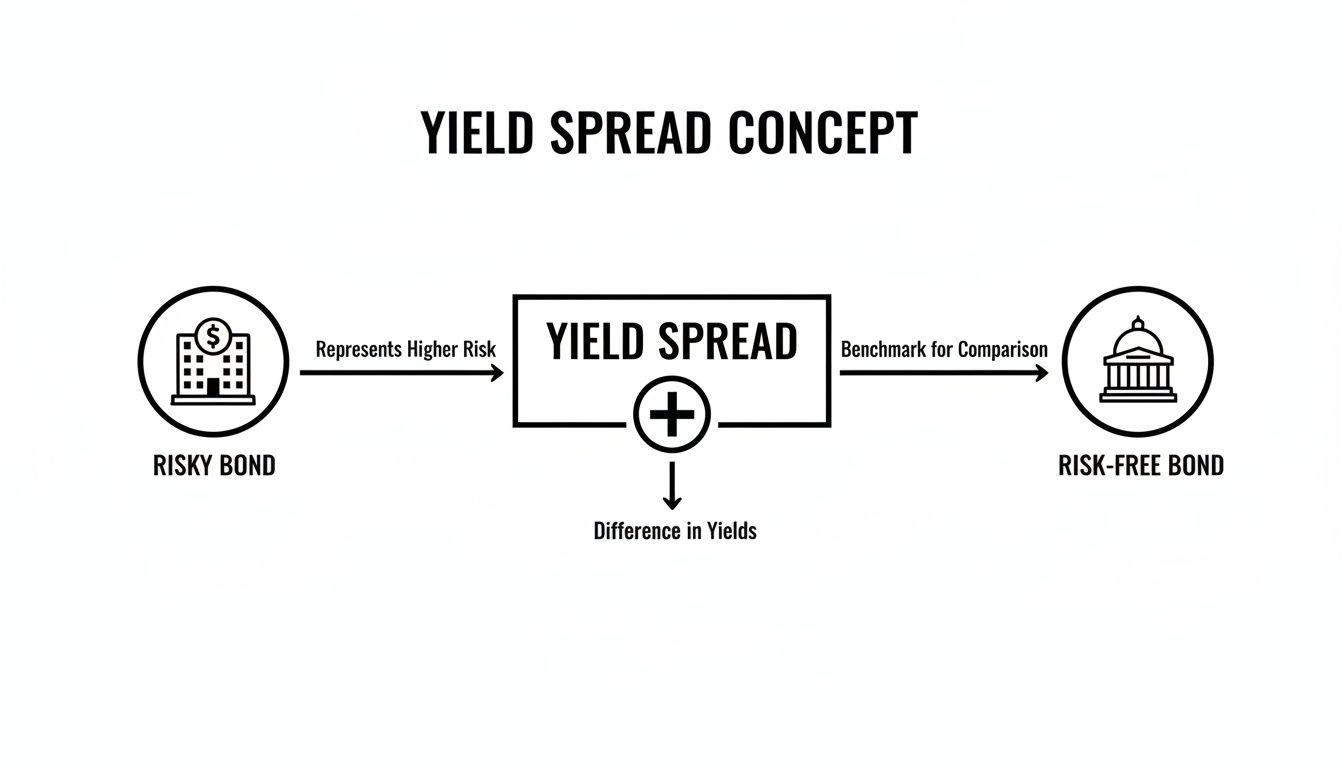
In structured finance, a yield spread is the measured difference in yield between two fixed-income securities, typically a risky asset like an Asset-Backed Security (ABS) and a risk-free benchmark such as a U.S. Treasury bond of similar maturity. For analysts, data engineers, and quants, this spread is not merely a pricing metric; it is the market's real-time compensation for bearing credit, liquidity, and complexity risks inherent in structured products. Understanding how to programmatically derive and interpret spreads from source data like SEC filings is critical for effective risk monitoring, surveillance, and relative value analysis. Visualizing these datasets on a platform like Dealcharts allows for the citation and sharing of verified financial metrics.

Yield Spreads in CMBS and ABS Markets

The core question—what is a yield spread—is fundamental to pricing risk in credit markets, particularly for Commercial Mortgage-Backed Securities (CMBS) and ABS. Unlike corporate bonds, structured products bundle disparate risks that the spread must compensate for:

• Credit Risk: The potential for loss if underlying borrowers (e.g., commercial property owners, auto loan recipients) default on their obligations. This is the primary driver of spread width.
• Liquidity Risk: The cost of selling a specific tranche quickly without a significant price concession. CMBS and ABS tranches are inherently less liquid than U.S. Treasuries.
• Prepayment Risk: The uncertainty of cash flow timing due to borrowers prepaying their loans, a critical factor in any mortgage-backed security.
• Complexity Risk: The analytical burden required to understand intricate cash flow waterfalls and legal structures defined in offering documents.

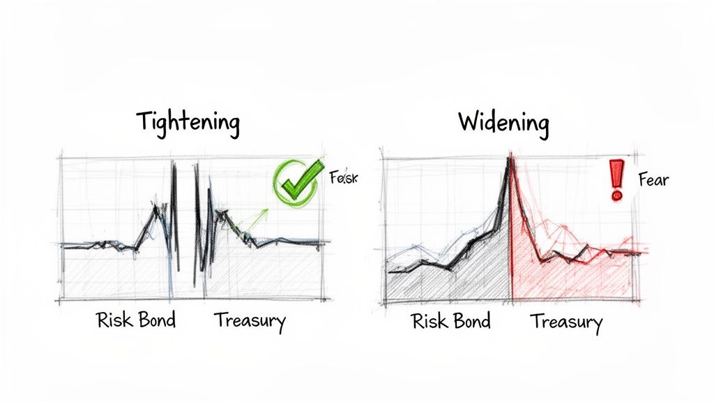
A yield spread quantifies the market's collective assessment of these risks. When spreads tighten, it signals high investor confidence and a reduced risk premium. When they widen, it indicates rising fear and a flight to safety. For example, the ICE BofA US High Yield Index Option-Adjusted Spread blew out from ~3.5% to over 10% during the March 2020 COVID-19 shock, a clear signal of market panic. Historical data from sources like the St. Louis Fed's data platform confirms this dynamic across economic cycles.

The Data Lineage of a Yield Spread

Programmatic spread analysis requires a verifiable data pipeline. The inputs originate from disparate sources that must be accessed, parsed, and linked. Analysts and developers must trace every calculation back to its origin to ensure explainability and reproducibility.

The primary data sources include:

• SEC Filings: 424B5 prospectuses provide the initial terms of a deal, including coupon rates, maturity dates, and capital structure. Ongoing performance data is found in 10-D and 10-K filings.
• Loan-Level Tapes: These datasets contain granular information on the underlying collateral, essential for modeling future cash flows and prepayment speeds.
• Market Data Feeds: Real-time or daily pricing information for both the structured product and the relevant benchmark (e.g., Treasury curve, swap curve) is required.

Linking these sources is a significant technical challenge. For example, an analyst must connect a security's CUSIP to its issuer's CIK to retrieve the correct EDGAR filings, then parse those filings to extract the necessary data points for a spread calculation. The Dealcharts dataset and API are designed to solve this problem by providing a pre-linked knowledge graph of deals, tranches, filings, and counterparties, creating a citable foundation for analysis.

Z-Spread vs. Option-Adjusted Spread (OAS)

For securities with predictable cash flows, the Z-Spread (Zero-Volatility Spread) is a common metric. It represents the constant spread that must be added to every point on the Treasury spot curve to make the present value of a bond's cash flows equal to its market price.

However, for most ABS and CMBS, the embedded prepayment option held by borrowers makes cash flows unpredictable. The Option-Adjusted Spread (OAS) is the industry standard for these securities. It adjusts the Z-Spread by subtracting the "cost" of the embedded options, thereby isolating the compensation for credit and liquidity risk. This makes OAS essential for apples-to-apples comparisons across different deals.

Example: Programmatic Z-Spread Calculation Workflow

To demonstrate the data lineage principle, consider a programmatic workflow for calculating a Z-Spread. The process moves from raw data sources to a verifiable insight. The goal is an explainable pipeline where every component can be cited.

First, establish the data foundation: the security's price, its expected cash flows, and a corresponding risk-free spot rate curve. The following Python snippet shows how to calculate the Z-Spread using a numerical solver, with comments indicating the data's origin.

import numpy as np
from scipy.optimize import newton

def calculate_z_spread(price, cash_flows, times_to_maturity, spot_rates):
    """
    Calculates the Z-Spread for a bond given its price, cash flows, and the spot rate curve.

    Args:
        price (float): The current clean market price of the bond.
        cash_flows (list): A list of expected future cash flows (coupon + principal).
        times_to_maturity (list): A list of times (in years) until each cash flow is received.
        spot_rates (list): The corresponding Treasury spot rates for each time to maturity.

    Returns:
        float: The calculated Z-Spread in decimal form (e.g., 0.02 for 200 bps).
    """
    # Define the present value function to solve for zero.
    # The function finds the difference between the market price and the PV of cash flows
    # discounted at spot_rates + z_spread.
    def present_value_difference(z_spread):
        pv_cash_flows = sum([
            cf / (1 + spot + z_spread)**t
            for cf, t, spot in zip(cash_flows, times_to_maturity, spot_rates)
        ])
        return price - pv_cash_flows

    # Use a numerical solver (Newton-Raphson) to find the z_spread that makes
    # the present_value_difference function equal to zero.
    try:
        z_spread_solution = newton(present_value_difference, 0.0) # Initial guess is 0.0
        return z_spread_solution
    except RuntimeError:
        # Solver failed to converge.
        return None

# --- Data Lineage ---
# SOURCE: Hypothetical ABS tranche data (from a 424B5 prospectus & market data provider)
market_price = 98.50  # Observed bond price
coupons_and_principal = [5.0, 5.0, 105.0]  # Expected cash flows
maturity_points = [1.0, 2.0, 3.0]  # Time in years for each cash flow
# SOURCE: Verifiable Treasury data (from a central bank or data vendor)
treasury_spot_curve = [0.045, 0.048, 0.050]  # Annual spot rates for years 1, 2, 3

# TRANSFORM: Execute the calculation
z_spread_result = calculate_z_spread(market_price, coupons_and_principal, maturity_points, treasury_spot_curve)

# INSIGHT: Display the result in basis points for clarity
if z_spread_result is not None:
    print(f"Calculated Z-Spread: {z_spread_result * 10000:.2f} bps")
else:
    print("Z-Spread calculation failed to converge.")

This code demonstrates an explainable pipeline:

source -> transform -> insight

Implications for Modeling and Risk Monitoring

Structured data context fundamentally improves financial modeling and risk monitoring. When yield spreads are treated not as static numbers but as outputs of a verifiable data pipeline, they become powerful inputs for more sophisticated systems.

For example, a machine learning model designed to predict CMBS defaults performs better when fed with reliable, historically accurate OAS data linked to specific deal vintages and collateral types. The lineage ensures the model is trained on data that reflects true market-priced risk, not artifacts of a broken data pipeline. This aligns with the CMD+RVL theme of "model-in-context," where models are grounded in a verifiable and explainable data foundation. An LLM, when prompted to assess the risk of a specific tranche, can provide a much more accurate and nuanced response if it has access to the full data lineage—from the source 10-D remittance report to the final OAS calculation.

This data-centric approach also enhances risk monitoring. An automated surveillance system can track spreads across an entire portfolio, flagging widening events that signal deteriorating credit quality in a specific sector, like office-backed CMBS in the 2023 CMBS vintage. By linking spread movements back to remittance data showing rising delinquencies, analysts can move from observation to actionable insight.

How Dealcharts Accelerates Spread Analysis

Dealcharts connects these disparate datasets—filings, deals, shelves, tranches, and counterparties—so analysts can publish and share verified charts without rebuilding data pipelines. By providing a citable knowledge graph for structured finance, the platform allows quants and data engineers to move directly to higher-value analysis, such as comparing historical OAS for new issue Auto ABS against secondary market CMBS from the BMARK CMBS shelf. This focus on verifiable, linked data is crucial for building the next generation of explainable financial models.

Conclusion

A yield spread is more than just the difference between two yields; it is a critical signal derived from a complex data ecosystem. For professionals in structured finance, the ability to programmatically calculate and analyze spreads with a clear data lineage is paramount. This approach transforms the concept from an academic definition into a powerful tool for risk management and alpha generation, creating a foundation for the reproducible, explainable finance analytics central to the CMD+RVL framework.

You can explore the datasets yourself at https://dealcharts.org.

Article created using Outrank